Standard Deviation and Standard Error Walk Into a Tea Stall

It’s a Friday morning. The fan turns slowly. The kettle hisses. Vijay has his thirty-day notebook open. He has computed two numbers, written them side by side in the margin, and is staring at them:

SD = 13 SE ≈ 2.4

Both numbers came out of the same 30 rows of data. Both are in units of customers per day. Both have the word standard in their name. And yet they are wildly different.

His phone buzzes. His cousin, finally: “How confident are you about the 87-customer average, brother?”

Vijay types back, “SD is 13.”

The reply comes immediately: “That’s not what I asked, Vijay. I asked about the average — not the days. You gave me the wrong number.”

Vijay scratches his head with the pen. “Wrong how? 13 is the spread. Same data.”

The next text: “Different question. Try again.”

He mutters, “Same data. Same units. But different questions need different spreads?”

The awning rustles.

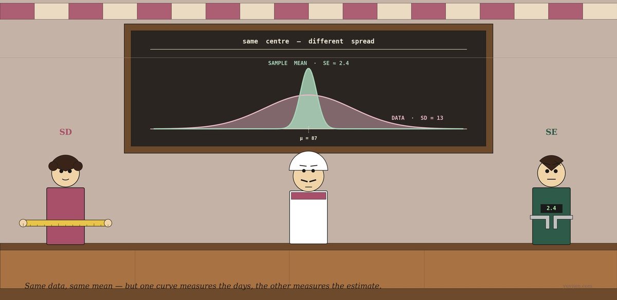
A woman steps in under the awning — brisk, bright cranberry shirt, hair in soft waves. In her two hands she holds a long yellow measuring tape, stretched out wide between them. The tape has tick marks every centimetre and a few longer ones at the fives.

She says, “I am Standard Deviation. People write me as SD or s or σ. I describe your data. How scattered are the individual days around their mean? My number, 13, says: a typical day differs from the average by about 13 customers.”

A man drifts in behind her — careful, settled, forest-green shirt, holding a small precision caliper in his right hand. The caliper’s jaws are pinched almost shut. A tiny digital readout on top blinks 2.4.

He says, “I am Standard Error. People write me as SE — or sometimes SEM, the standard error of the mean. I do not describe your data. I describe your estimate. If you ran another 30-day notebook, your sample mean would come out a little different. My number, 2.4, says: probably within about 2.4 customers of 87.”

Vijay says, “But you both have the word standard in your name. You both have units of customers. You both came out of my 30 rows.”

They reply, together, “Same input. Different question.”

SD speaks first

SD lays her tape across the counter. She says, “Look at your individual days. Some days you had 60 customers. Some days you had 108. Some days you had 91. They are not all 87. The average is 87, but the actual days are scattered around 87.”

Vijay nods.

“I measure that scatter. My number, 13, says: if I draw a band of ± 13 around 87 — so from 74 to 100 — most of your days fall within that band. Specifically, about 68% of them, if the data is roughly bell-shaped. ± 2 SD — from 61 to 113 — captures roughly 95% of the days.”

She pulls her tape wider, then narrower, then wider again. “I am a property of the data. If you collected more days, my number would barely change. The spread of individual days is what it is. More data doesn’t make the days less variable.”

Vijay says, “So you’re describing how scattered the actual data is.”

“Yes. I am descriptive. I describe what is there. The cousin is not asking me. He is asking him.”

She nods at SE.

SE speaks

SE sets his caliper on the counter. The digital readout glows steady at 2.4.

He says, “I describe something different. I describe how uncertain you are about the mean itself.”

He continues, “You computed a sample mean of 87 from 30 days. If you came back tomorrow and collected another 30 days — same stall, same season, same conditions — your sample mean would not be exactly 87. It might be 85. Or 89. Or 86.5. The sample mean is itself a random thing, because which 30 days you happen to collect is random.”

Vijay’s eyes widen.

“That randomness — the spread of the sample mean across hypothetical repeated samples — is what I measure. My number, 2.4, says: across all the possible thirty-day notebooks you could have collected, your sample mean would land within about ± 2.4 of the true mean most of the time.”

He picks up the caliper. “The relation is simple. SE = SD / √n. So 13 / √30 ≈ 2.37. I am SD divided by the square root of the sample size. And that is the magic.”

Vijay says, “What’s the magic?”

“As you collect more data, n grows. My number, SE, shrinks like 1/√n. If you collect 120 days instead of 30, my number drops from 2.4 to 1.2. Your estimate of the mean gets twice as precise.”

He pauses. “But SD does not change. The spread of individual days is what it is. More data just means you average over more wobbles, so the average becomes more stable. That’s the entire trick of statistics.”

What just happened

Vijay pours himself a glass of tea for the first time all morning, sits down on his own counter, and looks at the two of them.

He says, slowly, “So SD describes the days. SE describes my estimate of the average of the days.”

Both nod.

“And the cousin’s question — how confident are you about the average? — was asking about the estimate, not the data. So I should have answered SE ≈ 2.4, not SD = 13.”

Both nod again.

SD adds, “And it is much smaller — about √30 ≈ 5.5 times smaller. That is how much more confident you are about the mean than about any individual day. The averaging soaks up the noise.”

SE adds, “And every confidence interval you’ve ever seen is built on me. Mean ± 1.96 × SE for a 95% confidence interval (in the large-n limit). Mean ± t × SE for the t-distribution version, with t chosen from your degrees of freedom. The 1.96 and the t come from the distribution shape; I am the scale.”

Vijay says, “If I had answered the cousin’s question with 87 ± 13, that would have been an interval around the days, not around the mean. Wildly wide. Almost useless.”

SE: “Correct. 87 ± 2.4 is what he was asking for. Roughly: ‘the true average customer count is probably somewhere between 82 and 92, given my thirty days’.”

The same chat, in a chart

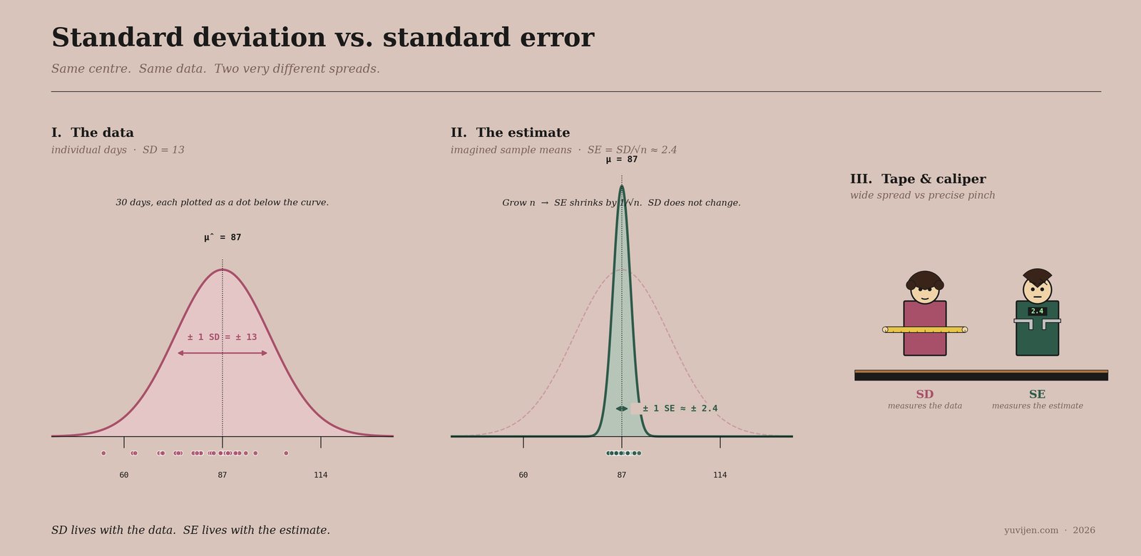
That picture is exactly the same conversation, drawn. The first panel is the data — 30 dots scattered widely, SD captures their spread. The second panel is the estimate — same x-axis, but a much narrower curve sits inside the faded ghost of the SD curve, and the imagined sample means cluster tightly. The third panel is SD and SE in person, holding their instruments: a wide tape for the wide spread, a precise caliper for the precise estimate.

One last warning before they leave

SD tucks her tape back into a coil. SE pockets his caliper. They look at Vijay together.

SE says, “Three traps.”

He counts them off.

“One. Error bars on charts. In a scientific paper or a dashboard, error bars can be SD or SE or a 95% confidence interval. They look identical. They mean different things. If the paper says mean ± SE, the bars look small and the result looks precise. If the paper says mean ± SD, the bars are huge and the variability looks alarming. Always check the caption. Many papers don’t even tell you which one — that’s a citation crime.”

SD adds, “Two. SE only describes the mean. People sometimes say SE of the data — that’s wrong. SE is always SE of an estimate. You can compute SE for a regression slope, an odds ratio, a proportion — any estimator. The general formula is SE(estimator) = SD(estimator across samples). The SE = SD / √n form is specific to the mean.”

SE adds, “Three. Don’t quote SE without n. SE = 2.4 sounds great. But if n = 4, that SE was computed from a tiny sample and is itself unreliable. If n = 10,000, the SE is rock-solid. Always quote n alongside SE. Otherwise the precision claim is unverifiable.”

Vijay nods. “SD for the data. SE for the estimate. Always check error-bar captions. Always quote n.”

Both confirm. “Yes.”

Quick gut-check

Three real scenarios. Do you want SD or SE?

1. “How much do customer counts vary from one day to the next at this stall?”
2. “What is the margin of error on the average customer count for the month?”
3. “Across many tea stalls in this city, how scattered is the typical daily-customer count?”

Scenario 1. SD — the question is about how individual days vary. Use the SD of the daily counts. The answer in Vijay’s case: 13 customers/day. Scenario 2. SE — the question is about the precision of the mean. Build the confidence interval with SE: mean ± 1.96 × SE. In Vijay’s case: 87 ± 4.7, so roughly 82 to 92. Scenario 3. SD again — same as scenario 1, just applied to a different population (stalls instead of days at one stall). The question is about the spread of individual values in the population, not about an estimate of a mean.

The pattern: SD is about individual values. SE is about an estimate. Almost every confidence interval and hypothesis test uses SE, because they’re about estimates. Descriptive statistics quoted as “typical ± typical wobble” use SD, because they’re about the data.

The bill

Vijay closed his notebook with a small smile. He had two numbers, side by side, in the margin: SD = 13 for the days, SE ≈ 2.4 for the mean. He had texted the cousin back the right number: 87 ± 2.4, approximately. The true average customer count is probably somewhere between 82 and 92.

The cousin had replied with the only thing he ever replied with when Vijay got it right: “Good.”

SD packed up her measuring tape and walked out under the awning, the tape coiled into a neat circle. SE pocketed his precision caliper, finished his tea in two careful sips, and left. The fan ticked. The kettle hissed. Vijay turned to a fresh page in his notebook and wrote, in the margin, the only sentence he wanted to remember from the visit:

SD describes the data. SE describes the estimate. SE = SD / √n. More data tightens SE, not SD.

His cousin, characteristically, texted one more thing: “Now go compute a confidence interval, brother. You have all the pieces.”

Vijay started a new page.

For the math-curious

Formal definitions: $s = \sqrt{\frac{1}{n-1} \sum_{i=1}^{n} (x_i - \bar{x})^2}$ is the sample standard deviation. It estimates the population SD σ.

$\text{SE}(\bar{x}) = \frac{s}{\sqrt{n}}$ is the standard error of the mean. It estimates the SD of the sampling distribution of x̄.

The 1/√n magic. The sampling distribution of the mean has standard deviation σ/√n exactly. As n grows, the sampling distribution gets tighter and tighter — by the Central Limit Theorem, it also gets more bell-shaped, regardless of what the data distribution looks like (as long as σ is finite). This is why the formula mean ± 1.96 × SE gives a roughly 95% confidence interval for almost any data, large enough n.

Confidence interval (95%, large n): $\bar{x} \pm 1.96 \cdot \text{SE} = \bar{x} \pm 1.96 \cdot \frac{s}{\sqrt{n}}$

For small n, use the t-distribution: $\bar{x} \pm t_{n-1,\, 0.025} \cdot \frac{s}{\sqrt{n}}$ where t_{n-1, 0.025} is the critical value of the t-distribution at df = n − 1 (see the Degrees of Freedom post for why n − 1).

Same data. Two spreads. SD belongs to the days. SE belongs to the mean.