Degrees of Freedom Walks Into a Tea Stall

It’s a Thursday afternoon. The fan turns slowly. Vijay has the calculator open and his thirty-day notebook beside it. He has been running t-tests for two weeks now — cardamom helped, ginger biscuits helped, the cousin’s claim about 100 was wrong. But today he has finally noticed a small pattern in every formula and every output, and it is bothering him.

The sample variance: divide by n − 1. Not n.

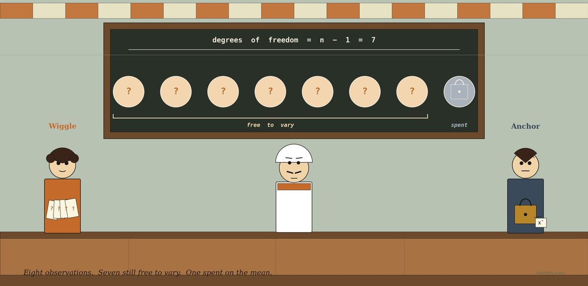
The t-distribution lookup: df = n − 1. Not n.

The two-sample t-test: df = n₁ + n₂ − 2. Always something minus.

He stares at the formulas. He mutters, “Why minus 1? I have 30 data points. Why does the formula act like I have 29?”

His phone buzzes. The cousin, late as always: “Brother, every time you compute something from the data, you pay for it with one of your data points. That’s degrees of freedom.”

Vijay reads it twice and is somehow more confused.

The awning rustles.

A woman steps in under the awning — bright, energetic, warm orange shirt, curly hair. In her right hand she has a small fan of blank slips of paper, each printed with a single ?. She holds them up like playing cards.

She says, “I am Wiggle. I am the freedom in your data. Out of your n observations, I am the ones that can take any value they like — given that the constraints you’ve placed on the data are respected.”

A man drifts in behind her — calm, settled, graphite-blue shirt, holding a small brass padlock in his right hand. A tiny paper tag dangles from the lock, and the tag reads x̄ in neat handwriting.

He says, “I am Anchor. I am the spent observation. The moment you compute the sample mean from your data, the last observation is no longer free — it is locked in to whatever value makes the mean come out right. I am the slot that has been used up.”

Vijay says, “But I have 30 rows. None of them is locked. They are all just… numbers I wrote down.”

They reply, together, “Until you compute the mean. After that, one of them is no longer free.”

Wiggle speaks first

Wiggle fans her slips out across the counter. Each one has a ? on it. She says, “Imagine your 30 rows as 30 slips. Before you compute anything, all 30 are free — they could be any number. The data is what it is.”

Vijay nods.

“Now — the moment you compute the sample mean and commit to it — the constraint kicks in. The 30 numbers must average to that mean. That is now true. Forever. Of those 30 numbers, 29 of them can still be whatever they were. But the 30th is forced to be the value that makes the average work out right.”

She looks at him. “I have n − 1 = 29 slips left in my hand. The 30th is gone. He took it.”

Anchor, behind her, lifts the padlock slightly.

Vijay says, slowly, “So the number of free slots is n − 1. Not because the 30th row physically changed — but because given the mean, the 30th row is determined by the other 29.”

“Exactly. I am the 29 free slots. He is the 1 spent slot. Together we are still n — but only n − 1 of us can be freely varied.”

Anchor speaks

Anchor sets the padlock on the counter. He says, “Let me give you the cleanest example. Forget your notebook. Imagine 4 friends sit down for tea. They get a single bill — ₹400. They want to split it however they like.”

Vijay says, “OK.”

“Friend 1 throws in ₹100. Friend 2 throws in ₹80. Friend 3 throws in ₹150. Each picks freely. No constraint yet — the totals so far are ₹330.”

He pauses.

“Friend 4 cannot pick freely. Friend 4 must pay ₹70. The bill is ₹400. The other three have already paid ₹330. The 4th person’s share is locked in by the constraint that the total equal ₹400.”

Vijay watches him carefully.

“4 friends. 1 constraint (the total bill). 3 of them free to pick. Degrees of freedom: n − 1 = 3. That is the entire idea.”

He nods at Wiggle. “When you compute the sample mean from n data points, you have done the same thing. The mean is a constraint — it says the sum of these numbers must be n × mean. With that constraint in place, only n − 1 of the original numbers can be freely varied. The n-th is determined.”

Vijay sits down on his counter and pours himself a glass of tea.

He says, “So degrees of freedom is just the number of values that can still wiggle, after the constraints are imposed.”

Both nod. “Yes.”

What just happened

Vijay says, “And every parameter I estimate from the data is a constraint. The mean is one constraint. So I lose one degree.”

Anchor: “Yes.”

Vijay: “If I estimate two parameters — say a regression slope and an intercept — I lose two degrees.”

Anchor: “Yes. Simple linear regression has df = n − 2.”

Vijay: “If I run a two-sample t-test, I estimate two means — one per group. So I lose two degrees, total. df = n₁ + n₂ − 2.”

Wiggle nods, smiling. “You see the pattern. df = n − p, where p is the number of parameters you’ve estimated. It’s not magic. It’s bookkeeping.”

Vijay says, “Why does the calculator divide by n − 1 for sample variance? Same reason?”

Anchor: “Same reason. To compute sample variance, you first compute the mean. So when you sum up the squared deviations from the mean, only n − 1 of those deviations are free. The n-th is determined. Dividing by n − 1 corrects for that — it gives you an unbiased estimate. Dividing by n would systematically underestimate the true variance.”

Vijay nods. “So n − 1 isn’t a tradition. It’s a correction.”

“The correction is called Bessel’s correction. Friedrich Bessel, German astronomer, 1840-something. Every introductory stats book divides by n − 1 because of him.”

The same chat, in a chart

That picture is exactly the same conversation, drawn. The first panel is the slot view: n observations, one of them spent on the mean, leaving n − 1 free to vary. The second panel is the bill-splitting view: a known total turns one of four free numbers into a determined number, leaving 3 degrees of freedom. The third panel is Wiggle and Anchor in person — the free slips and the locked padlock, side by side.

One last warning before they leave

Anchor packs the padlock back into his pocket. He says, “Three traps.”

He counts them off.

“One. Different tests have different df formulas, because they estimate different numbers of parameters. One-sample t-test: df = n − 1. Two-sample t-test (pooled): df = n₁ + n₂ − 2. Simple linear regression: df = n − 2. Multiple regression with k predictors plus intercept: df = n − k − 1. Chi-square test on a contingency table with r rows and c columns: df = (r − 1)(c − 1). Don’t memorise the formulas — memorise the rule: count parameters estimated, subtract.”

Wiggle adds, “Two. Smaller df means a fatter t-distribution. The t-distribution at df = 2 has dramatically heavier tails than the standard normal. As df grows, the t-curve approaches the standard normal — by df = 30 they’re nearly identical, by df = 100 they’re indistinguishable in practice. That is why small samples need wider confidence intervals: you have fewer free observations, so your variance estimate is shakier, so you need a larger margin.”

Anchor: “Three. Don’t mix up the df reported by software with the number of observations. If your spreadsheet reports df = 28 for a two-sample t-test, that’s n₁ + n₂ − 2 = 28, which means you had 30 total observations. The number you write in your methods section should be the count, not the df. Confusing them shows up in regression tables more often than people admit.”

Vijay nods. “Count parameters. Subtract. Don’t mix df with n.”

Both confirm. “Yes.”

Quick gut-check

Three real scenarios. What’s the df?

1. A one-sample t-test on 25 customer ratings, comparing the mean to a fixed claim of 4.0 stars.
2. A simple linear regression of daily sales on outdoor temperature, fitted to 40 days of data. The model has an intercept and one slope.
3. A chi-square test of independence on a 3 × 4 contingency table — three product types, four regions.

Scenario 1. df = 24 — that is n − 1 for a one-sample t-test (25 − 1). Scenario 2. df = 38 — for the residuals of simple linear regression, that’s n − k − 1 = 40 − 1 − 1 = 38 where k = 1 predictor (temperature) and the + 1 is the intercept. Scenario 3. df = 6 — for chi-square on an r × c table, df = (r − 1)(c − 1) = (3 − 1)(4 − 1) = 2 × 3 = 6. Notice that for the chi-square the formula isn’t n − p — chi-square on contingency tables uses the dimensions of the table, not the number of cells. Different test family, different bookkeeping. Same underlying idea: count what’s free, given the constraints.

The trick is to ask: what constraints have I imposed on the data by estimating parameters? Each constraint costs you one slot. The answer is what’s left.

The bill

Vijay closed his notebook with a small smile. He had 30 rows. He had n − 1 = 29 degrees of freedom for his one-sample t-test. The cousin’s text had been right, in his bluff way: every parameter he estimated cost him one of his data points. Bessel’s 1820-something correction was the math admitting that fact honestly.

Wiggle gathered her fan of blank slips and tucked them into a satchel. Anchor pocketed the brass padlock — the x̄ tag swung against the metal as he walked. The fan ticked. The kettle hissed. Vijay turned to a fresh page in his notebook and wrote, in the margin, the only sentence he wanted to remember from the visit:

Degrees of freedom = n − (parameters estimated). Every constraint costs one slot. The math just keeps the books.

His cousin texted again, perfectly timed: “Did you get it now?”

Vijay typed back, “You took one of my data points.”

The cousin, characteristically, did not reply.

For the math-curious

Formal definition: For a statistic computed from n observations with p independently estimated parameters, $\text{df} = n - p$

df for the common tests: – One-sample t-test: df = n − 1 (estimating one parameter — the mean) – Two-sample t-test, pooled: df = n₁ + n₂ − 2 (estimating two means) – Welch’s t-test (unequal variances): df is non-integer, computed by the Welch–Satterthwaite equation — software handles it – Paired t-test: df = n − 1 where n is the number of pairs (treats differences as a one-sample test) – One-way ANOVA: numerator df = k − 1 (between-groups, k = group count); denominator df = N − k – Simple linear regression: residual df = n − 2 – Multiple regression with k predictors: residual df = n − k − 1 – Chi-square test of independence on r × c table: df = (r − 1)(c − 1) – Chi-square goodness-of-fit on k categories: df = k − 1 (or k − 1 − p if you also estimated p parameters)

The connection to fatter t-tails: The t-distribution at df → ∞ is exactly the standard normal. At df = 30, the difference is small. At df = 5, the t-distribution has visibly heavier tails — meaning the critical value for α = 0.05 (two-sided) is 2.57 instead of the normal’s 1.96. Smaller df → fatter tails → more cautious test.

Same idea, every time. Count what’s free, given what’s been spent.