
It’s a hot afternoon. The kettle hisses. The ceiling fan turns slowly above. Vijay has reopened his thirty-day notebook. Daily customer counts down one column. He has computed the average: 87.
His cousin (who has, this month, theorised that the moon affects sweet sales and that hotter days mean more tea) has been telling him for weeks: “Brother, your stall should average 100 customers a day. That’s the right number. You are losing somewhere.”
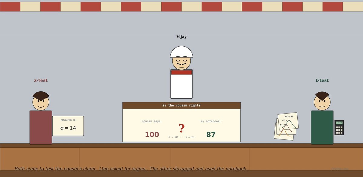
Vijay does not know whether 87 is meaningfully below 100 or whether the gap is just sampling noise — some weeks busier, some quieter, the mean wobbles. He needs a test. He has heard there are two. He does not know which.
He mutters, “Same data. Same question. Why are there two tests?”
The awning rustles.
A woman steps in under the awning — neat, confident, holding a small printed index card. The card has just one thing written on it in big serif type: σ = 14. She places it lightly on the counter and says, “I am z-test. Tell me what sigma is. I’ll plug it in. Done.”
A man steps in behind her — careful, slightly self-deprecating, holding three things at once: Vijay’s notebook (which he picked up from the counter on his way in), a small handheld calculator, and a tiny fan of bell-curve cutouts in his other hand — three small cards each printed with a different bell shape, labelled df = 2, df = 10, df = 30. He sets the fan down beside the notebook and says, “I am t-test. I do not know sigma. I’ll estimate it from your numbers — and because I’m estimating, I’ll be a little more cautious. Especially when your notebook is small.”
Vijay looks at them, looks at his card, and asks, “Which one of you do I need?”
They reply in unison: “Probably him.” Then z-test adds, “But it would be polite to explain why.”
z-test tries first
z-test picks up Vijay’s notebook and squints at the columns. She says, “I work like this. Your sample mean is 87. The cousin’s claim is 100. The gap is 13. Now I divide that gap by the standard error — sigma over root-n. Plug in sigma, plug in n, look up the answer in the standard normal table. Reject or fail to reject.”
Vijay nods. “And sigma is…”
She pauses. “Sigma is the population standard deviation. The true spread of customers per day across every possible day, sunny or stormy, festival or Tuesday. The whole population.”
Vijay says, “I… only have thirty days written down. I do not know that.”
She frowns. “Then I cannot really do this cleanly. I work when sigma is given to you — when someone has already measured the whole population and handed you the value.” She taps her card, where it still reads σ = 14. “If you knew that, I’d be your test. You don’t.”
She looks at t-test, who is already opening Vijay’s notebook with a small smile.
t-test tries
t-test sets the notebook flat on the counter and runs his eyes down the customer-count column. He picks up his calculator. He punches in numbers for a minute. Then he writes, on a corner of newspaper:
sample mean: 87 sample standard deviation: 13 n: 30
He says, “I do not know sigma. So I use s — the sample standard deviation, computed from your thirty days. It is an estimate of sigma, not sigma itself.”
He looks at his calculator. “Standard error is s ÷ √n = 13 ÷ √30 ≈ 2.4. Test statistic is the gap divided by that standard error: (87 − 100) ÷ 2.4 ≈ −5.31.”
He picks up the bell-curve fan and looks at it carefully. He pulls out the card labelled df = 29. (Degrees of freedom = n − 1 = 29.) “This is the curve I look up against. The t-distribution at twenty-nine degrees of freedom.”
He writes one more line:
t = −5.31, df = 29, p < 0.001
He says, “The cousin is wrong. Reject. The data really does sit far below 100 — by far more than sampling noise can explain.”
Vijay leans in. “And if I’d had a small notebook? Five days, not thirty?”
t-test sighs the patient sigh of a man who has explained this many times. “Then I would have used a fatter curve from my fan — df = 4, much heavier tails — and I might have failed to reject. Less data, more uncertainty, more cautious test.”
z-test, slightly defensive, adds, “And I would have been overconfident on the same five days. I would have used the standard normal — thin tails — and given you a smaller p-value than I deserved.”
What just happened
Vijay pours himself a glass of tea for the first time all afternoon, sits down on his own counter, and asks, “So both of you compare the gap between sample mean and the cousin’s claim — divided by the standard error. Same arithmetic so far.”
Both nod.
“But you” — he points at z-test — “use sigma, the population SD. And you” — he points at t-test — “use s, the sample SD.”
t-test says, “Yes. And because s is an estimate, it has its own uncertainty, especially when n is small. The t-distribution is fatter in the tails than the normal — it gives you more room for that uncertainty. As n grows large, the fatness goes away. By the time you have a hundred rows, the two of us give the same answer to four decimal places.”
He pauses, then adds quietly, “Also — you wouldn’t know my real name. I was invented at the Guinness brewery in Dublin in 1908. The man who created me — William Sealy Gosset — published as Student because Guinness would not let employees publish under their own names. The ‘Student’s t-test’ you read about in textbooks is named after a brewery’s company policy.”
Vijay raises his glass. “To Student.”
z-test sniffs. “I am older. Gauss. Eighteenth century.”
t-test says, “And you are correct, when σ is known. It is just that, for the rest of us, σ is almost never known.”
The same chat, in a chart

That picture is exactly the same conversation, drawn. The first panel shows what the two distributions actually look like — the t-distribution at small df has visibly fatter tails, and by df = 30 it sits almost on top of the standard normal. The second panel shows Vijay’s data: at n = 30, both tests reject the cousin (p < 0.001); at n = 5, the same test statistic gives p ≈ 0.12 from the t-test (don’t reject) but p ≈ 0.05 from the z-test (reject) — they disagree, and the t-test is correctly the cautious one.
One last warning before they leave
t-test packs his calculator back into his shirt pocket. He says, “One thing, Vijay. The most common mistake is using me for proportions instead of means. I am for the mean of a continuous variable. For proportions — what fraction of customers buy a samosa — there is a different test (z-test for proportions, despite the name, since the central limit theorem makes the proportion’s sampling distribution roughly normal for large n). Don’t bring me to a proportion problem and expect a clean answer.”
z-test adds, “And don’t use me — the z-test — just because n is large. Yes, by n > 30 we mostly agree. But the principled choice is based on whether sigma is known, not on sample size. If sigma is estimated, even from a giant sample, the t-test is still the right framework. We just happen to give the same answer.”
Vijay nods slowly. “Use the t-test when I’m estimating sigma. Use the z-test only when sigma is genuinely given to me. And don’t use either one for proportions without checking.”
t-test says, “And remember why my distribution exists. Estimating sigma adds uncertainty. The fatter tails are how I respect that.”
Quick gut-check
You’re testing three claims at your tea stall. Which test would you reach for?
- “My average daily samosa sales is significantly different from 50. I have a notebook of 40 days.”
- “Forty per cent of my customers order biscuits with their tea — is the actual rate different from that?”
- “The mean filling weight of my mass-produced supplier’s biscuit pack is supposed to be 200g — the manufacturer publishes σ = 5g. I weighed 12 packs.”
1 is a t-test (mean, σ unknown, estimated from your forty-day notebook). 2 is a z-test for proportions (the rate 40% is a proportion, not a mean). 3 is a z-test of the mean — σ is given to you by the manufacturer.
The bill
Vijay closed his notebook with a small smile. The cousin’s 100 claim was rejected. The data really was at 87, and the gap was real — bigger than noise. Whatever the cousin had been theorising about, the math did not back him up.
The fan ticked. The kettle hissed. z-test tucked her σ = 14 card back into her sleeve. t-test folded his bell-curve fan, pocketed his calculator, finished his tea, and left a tip that worked out to a precisely-calculated fourteen per cent. He looked back from the awning and waved.
Use them together. z-test for the rare textbook case where sigma is known. t-test for almost everything else. Neither for proportions without thinking. And when in doubt — when you’re estimating sigma from your sample — the t-test is the cautious, correct choice.
For the math-curious
z = (x̄ − μ₀) / (σ / √n) — standard normal, σ known.
t = (x̄ − μ₀) / (s / √n) — Student’s t-distribution at
df = n − 1, with σ estimated as the sample SDs.As n grows, the t-distribution converges to the standard normal. By
n = 30the difference is small; byn = 100the two tests agree on practically everything. Belown = 30, always use the t-test if σ is estimated.
Same arithmetic. Different distribution behind the table you look up.